Dual-comb spectroscopy – KerrFrequencyCombs.org

The dual-comb approach (also called multiheterodyne approach) that is used in dual-comb spectroscopy^1,2 allows for fast and precise scans over a broad frequency (or wavelength) range without any moving parts. While this technique can of course be used for spectroscopy^3–5 it has by now found many more applications where it can replace scanning lasers and conventional broad-band light sources and optics. Examples are distance measurements (lidar)⁶ and rapid spatial scanning for imaging^7,19. Here we will look into a few aspects of dual-comb schemes and why Kerr frequency combs are a very suitable light source.

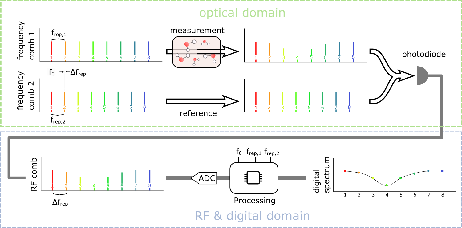
The basic idea is shown in the image above with a spectroscopy application. The essential requirement for dual-comb spectroscopy (DCS) are two frequency combs whose repetition rates (f_rep,1 and f_rep,2) are mismatched by a small amount (Δf_rep = f_rep,1 – f_rep,2). Assuming for simplicity that the lowest relevant frequency comb teeth of comb 1 and comb 2 with n = 0 are at the same frequency f₀, then all tooth pairs with identical n at higher frequencies (f_1,n = f₀ + n·f_rep,1 and f_2,n = f₀ + n·f_rep,2) have a difference that grows as n·Δf_rep. If after a beam combiner the two combs are detected on one sufficiently fast photodiode, these beat frequencies will represent a radio frequency (RF) comb with spacing Δf_rep in the electrical domain. The important part is that the frequencies in the optical domain and the frequencies in the RF domain have a one-to-one correspondence. Sampling the RF signal of the photodiode is therefore sufficient to obtain the changes in amplitude (and potentially phase) of the optical comb teeth, which is the wanted spectroscopic data.

In contrast to conventional spectroscopy techniques, neither moving parts (such as in typical FTIR spectrometers) nor specific optical elements (such as gratings) are required to spread the optical spectrum and to separate the optical frequencies. The separation is done in the electrical RF domain only and typically after digitizing the RF signal. As a result the optical beam path can be very simple and it can be fully implemented in optical fibers or even on a photonic chip. This simplicity is one of the main advantages of the dual-comb spectroscopy as it can allow for small, fast and robust spectrometers.

However, because the frequency separation is moved from the optical to the electrical domain the complexity of the signal processing is much higher in the electrical/digital domain compared to a conventional spectrometer. In a typical grating-based spectrometer with medium exposure times, the electronic design focuses on low additional noise. Speed is not an issue and the spectrum is very much valid right after readout as the calibration and averaging is done in the optical domain before the readout. In the dual-comb approach however, the full electronic and digital path has to be fast enough to support the beat signals which typically are in the range of tens of MHz to tens of GHz. In additional there is very little coherent averaging and no calibration happening in the optical domain. As a consequence, once the analog RF signal is sampled, rather complicated processing steps have to be undertaken before the spectrum is available. The difference of what is done in the optical domain and what is done in the electrical domain is shown below.

	Grating spectrometer	Dual-comb spectrometer
Optical	– sample interaction – separation of frequencies – averaging – calibration	– sample interaction
Electrical /Digital	– data acquisition and storage – limited post-processing	– data acquisition – separation of frequencies – averaging – calibration – data storage – post-processing

The calibration aspect included in the table stands for the calibration of the measurement with respect to a known frequency reference. When looking at the frequencies involved in the dual-comb scheme, only f₀ is in the optical domain. The two repetition rates are in the RF domain and can therefore be easily referenced against usual frequency standards. Therefore, if f₀ is known, the full spectrum can be calibrated in the post processing stage using the knowledge of the repetition rates. To obtain the maximum in precision and stability, it would be possible to derive f₀ of the frequency combs using the self-referencing technique, which made frequency combs the popular metrological tool that they are today⁸. While self-referencing does require substantial additional efforts, it is easier to implement with the dual-comb scheme compared to other spectroscopy approaches as there are already frequency comb sources present in the system.

From what is said above it is possible to state a few typical advantages and disadvantages of dual-comb spectroscopy compared to other techniques:

Advantages:

possibility for very fast measurements
potential for high reliability and robustness as no moving parts or large optical elements are involved
in principle very simple optical measurement setup (if frequency comb source is excluded), barely mechanical parts required
potential for very precise measurements due to RF referencing, including optical phases
potential for optical integration, even in photonic integrated circuits
if fully compensated, robust against external perturbations, drifts etc.

Disadvantage:

requires two rather sophisticated optical frequency comb sources
optical measurement range and resolution determined by frequency comb source
fast analog and digital RF circuits required
high signal-to-noise ratios only with averaging which requires either stabilization or compensation and reduced speed
full compensation requires sophisticated digital processing (e.g. FPGA) or stabilization setups

An example in numbers

Just to highlight a few key properties and relations of the dual-comb spectroscopy technique, here is an example scheme for a dual-comb spectrometer (wavelength is assumed to be around 1550 nm but it is not really important):
f_rep,1 = 100 MHz
f_rep,2 = 100.1 MHz
f₀ = 193 THz
One key parameter of this spectrometer is already defined by the repetition rates: the resolution. Because every frequency comb line will result in one data point at the frequency of this line, the distance between the points and therefore the resolution of the spectrometer is given by the repetition rate. therefore the resolution is 100 MHz. From the two repetition rates, it follow that Δf_rep is 100 kHz, which defines the spacing of the frequency comb in the RF domain after detection. This has two consequences. First, the measurement time has to be sufficiently long to resolve 100 kHz differences. Therefore it is at least 1/100kHz = 10 µs. Second, it gives the maximum number of lines n_max and therefore the maximum span of the measurement (n_max f_rep) because only for numbers below n_max the correspondence of RF frequency comb lines to the optical frequency comb lines remains unique. Once n_max Δf_rep becomes larger than f_rep/2 it becomes impossible to distinguish individual lines in the RF domain which means a direct mapping of RF frequencies to optical frequencies is not possible anymore (at least not for a measurement time of 1/Δf_rep). Therefore this poses a limit at n_max = f_rep/(2Δf_rep). For our example this means that one can resolve 500 lines. The full measurement span is then given as 500 f_rep = 50 GHz (e.g. < 0.5 nm at 1550 nm). If Δf_rep was only 100 Hz, the possible measurement range would multiply by this factor of 1000 to 50 THz, which is very significant. However, also the required measurement time would be substantially higher with a minimum scan time of 10 ms. Furthermore the changes of the repetition rates within this measurement time have to be limited to well below 100 Hz.

Finding the right balance between optics and electronics

For me one of the most interesting aspects in dual-comb spectroscopy is to find the right balance between the optics and the electronics. Quite some of the challenges involved in designing a working dual comb spectrometer involve working with both. As mentioned above, a basic requirement for a dual-comb spectrometer is to have two optical frequency comb sources with slightly different repetition rates. While it is easy to write down the frequencies of all lines of the two frequency combs in theory (see above), a real frequency comb does deviate from this. If a frequency comb is not fully stabilized and self-referenced, the two frequencies, f₀ and f_rep drift and jitter by some amount. Because of this the exact determination of Δf_rep is difficult and its value will change over time and in particular it can change over the measurement time. However, Δf_rep is a crucial parameter, as it was also shown in the example above, and it typically is much smaller than f_rep. Therefore even small deviations of the frequencies lead to problems and uncertainties in the data analysis, if they are not compensated.

This is where electronics comes into play. A part of the dual-comb spectrometer work relies on the stabilization of the frequency combs with external RF references to minimize the drift and jitter and to achieve a long coherence time⁹. Frequency stabilization is a very common technique and in particular in metrology it is heavily used for example for laser stabilization and self-referenced, stabilized frequency combs. For DCS typically one comb offset f₀ is locked onto the other and the two different repetition rates are locked to the same RF reference. The idea of this locking is to measure any small deviation of the stabilized frequencies and provide an actuation which compensates this deviations in order to keep the resulting error smaller than the required measurement accuracy. However, it is not always easy to achieve good stability and a typical setup for frequency stabilization requires several additional components in particular a servo controller and a sufficiently fast feedback (or feed-forward¹⁰) actuation. This can make the former simple optical setup rather complicated but it can also result in extremely precise spectroscopic measurements.

Increasingly it becomes therefore common to only track the changes and compensate them digitally^4,11,12. This requires neither servo controllers nor feedback mechanisms but only the ability to measure and process all changes in real time against a reference. In the simplest case this means that there are additional photodiodes and ADCs to measure and record the offset between the two frequency combs as well as the two repetition rates against a single RF reference. In a later step all this data is used to correct the RF signal of the two frequency combs. The complexity of additional hardware in the setup is therefore transferred to the digital and software domain which can be handled in real time by FPGAs. This can leads to more compact and potentially cheaper systems.

Both of the approaches, the full stabilization as well as only digital tracking, have their advantages and disadvantages. For example, in the latter approach it might become problematic if the optical frequencies drift too much such that a particular feature, that is supposed to be measured, is not properly probed anymore. This can not be compensated for digitally. Also the requirements for the two approaches are quite different. However, combinations are possible and are realized. Finding the best solution here depends very much on the exact system, the frequencies involved and the requirements.

Advantages of Kerr frequency combs

In the context of DCS Kerr frequency combs have a few potential advantages compared to « normal » frequency combs derived from mode-locked lasers. One crucial difference is that Kerr frequency combs allow large repetition rates up to hundreds of GHz. Theoretically this allows to measure extremely fast. Assuming f_rep = 50 GHz and 100 comb lines, a full spectrum could be acquired in 2·100/50 GHz = 4 ns. The optical resolution would then be given by the line spacing of 50 GHz (equivalent to 1.7cm^‒1 ~ 0.4 nm at 1550nm or 0.8 nm at 3 µm) and the measurement span is100 · 50 GHz = 5 THz (e.g. from 2925 nm to 3075 nm). One issue with these fast acquisitions is the SNR². Typically several measurements are averaged which increases the acquisition time. Nevertheless, the advantage in acquisition speed has been demonstrated in distance measurement experiments¹³. Depending on the averaging, the measurement error was between 280 nm at 100 MHz measuring rate (or 10 ns per point) and 12 nm for 75 kHz (13 µs per point).

Another advantage of Kerr frequency combs is that coherence between the two frequency combs can be guaranteed if the same pump laser is used for the generation of both frequency combs. This makes the scheme more robust and can simplify the spectrometer. This principle has been demonstrated. It is even possible to generate the two frequency combs in the same microresonator¹⁴. Something similar has also been shown for other types of laser systems¹⁵. Having one common cavity for the two lasers helps as much of the drift and noise sources are common (e.g. thermal drift of the cavity lengths) and can therefore be compensated easier.

The possibility of generating both frequency combs with different repetition rates in the same microresonator cavity highlights one more advantage: the very basic, fundamental setup to generate a Kerr frequency comb is fairly simple as it consists of only a continuous wave laser and a microresonator. And by now some Kerr frequency comb experiments do indeed start to deliver on this promise of simplicity¹⁸.

One promise of the on-chip platforms for Kerr frequency comb generation (such as waveguide resonators of any material or silica disks) is the photonic integration. While this is an intriguing perspective, integrating all parts required for a dual-comb setup onto one chip is challenging and has not been achieved in any setting so far.

And of electro-optic modulation combs

Some of the advantages given above are shared between Kerr frequency combs and electro-optic modulation (EOM) frequency combs^5,16,17. In particular, also EOM combs are derived from one cw laser and also the spacing of EOM combs can easily reach values around a few tens of GHz (but not the hundreds of GHz Kerr frequency combs can achieve). Additionally, EOM combs can substantially change their line spacings on the fly, something that neither mode-locked lasers nor Kerr frequency combs can do. Also the width of EOM combs can be adapted by changing the driving power of the modulators. However, these advantages are gained by having a non-resonant system which results in rather large power requirements for the modulators.

Commercial status and applications

Dual frequency comb spectrometers are a fairly hot research topic. However, there are companies which do already offer products based on the dual-comb approach. IRSweep makes a spectrometers which is positioned as a replacement for conventional mechanical FTIR spectrometers. MenloSystems offers a dual-comb system for different scientific applications.

Some different applications have been demonstrated using Kerr frequency combs and the dual-comb approach. Have a look here for relevant publications.

References

Because this is not a full review paper, the references are fairly selective and mostly from recent papers. For a more comprehensive list of references have a look at the relatively recent review paper by Coddington et al. in Optica (Open Access).

This work is licensed under a Creative Commons Attribution 4.0 International License.